
 Photo by Arian Korte on Unsplash
The Problem
Problem Description
The goal of this project is to build a machine learning model that processes audio files (in wav format for this particular case) and classifies them into the correct music genre.
Different types of machine learning solutions and algorithms are able to solve this problem, from Recurrent Neural Networks, in the form of LSTMs (Long Short Term Memory networks)[3], to Convolutional Neural Networks (CNN). For this particular project, I focus on building a CNN that can accurately predict the genre of different audio files.
The rest of the sections explain the different steps taken to arrive at a solid solution that can classify music with 87% of accuracy in the training set, and 87% accuracy in the validation/test set. To arrive at this solution several steps, described in the following sections, were taken. From extracting meaningful features to input to the CNN, to designing the CNN, to tuning the hyperparameters of the network.
There is a last section, called “How did I get here?” where I explained all the things that went wrong, that were later fixed. Everything from data augmentation, to avoiding overfitting, to increasing even more the accuracy, etc. I see that last section as things to remember when building machine learning solutions, and in particular deep learning solutions.
On the technical side, the following libraries were used: librosa, tensorflow together with keras, and the usual NumPy, and matplotlib for creating some graphs. All the code is available in GitHub, here.
This report has been written in Mardown and converted to pdf using pandoc, through a LaTex engine. The following command was used:
pandoc report.md --pdf-engine=xelatex -o report.pdf
The Data
Data Description
The GTZAN dataset is used for this project, very popular within the Music Information Retrieval community. Obtained from here and downloaded from here.
This dataset has a total of 10 different music genres: pop, metal, disco, blues, reggae, classical, rock, hiphop, country, jazz. Each genre has 100 audio files, where each file is of 30 seconds long. The total number of files is 1,000.
An extract from a blues .wav file is shown in Figure 1.
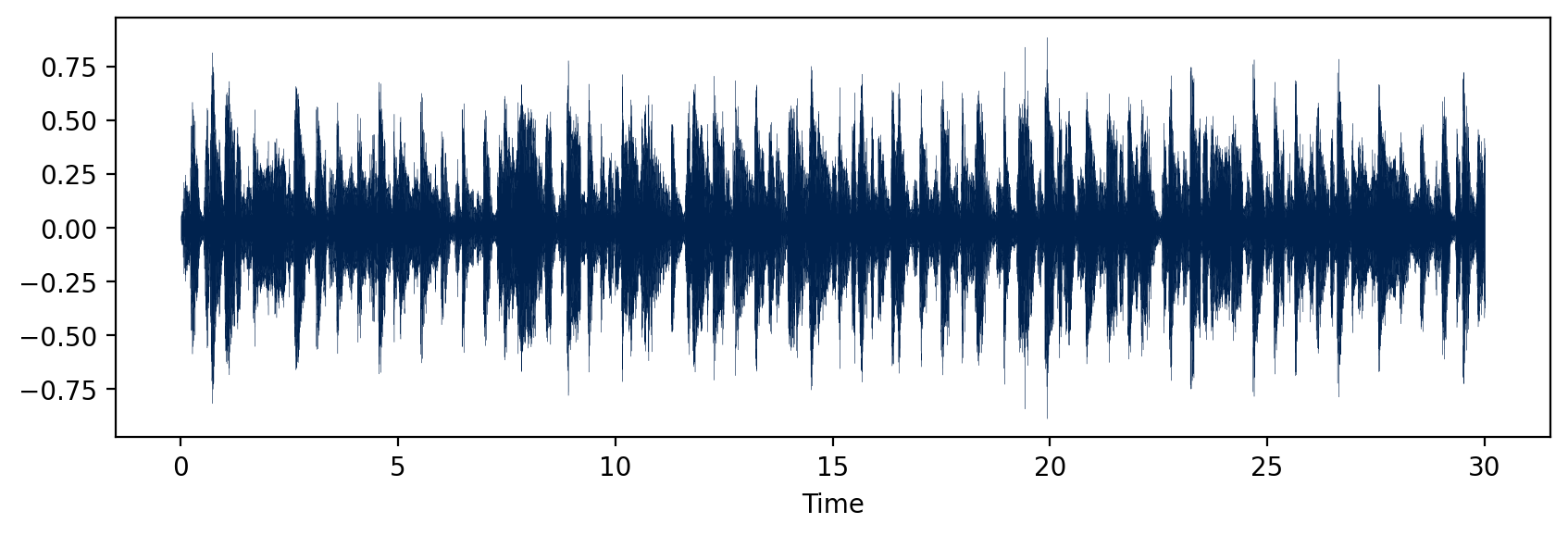
To process the data in python I have used the librosa library, where one can trim the signal, obtain the spectogram, and many more fun tricks.
The Features
Feature Engineering – Data Augmentation
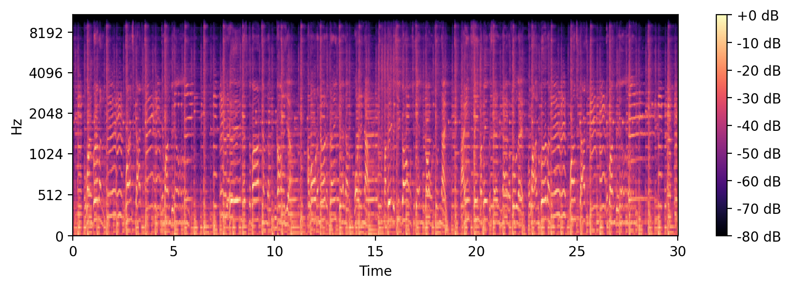
The question that I am trying to answer is: How can I construct features that will give enriched information for the CNN to interpret and try to learn from? Using librosa meaningful features can be extracted from audio data, such as Mel-frequency cepstral coefficients (MFCCs), Spectral Centroid, etc. I ended up deciding for a mel-spaced spectogram, that does a linear transformation to the signal, on the frequency domain, to present the frequency in a scale that is more noticeable for the human ear. It then computes a spectogram of that new scaled frequencies, yielding visual representations of the spectrum of frequencies, and their intensity.
That was exactly what I was looking for, since I was looking for features that resembled visual representations of the signal, since visual features is what CNNs are good at learning from. An example of the mel-spectogram from the signal from Figure 1 is shown in Figure 2.
Once I had that covered, the next point to take into consideration is the small dataset that I have. As a first try I tried learning from the different spectograms from the original data, using the CNN, but it was overfitting extremely easily. So I decided to use Data Augmentation to increase the size of the dataset, helping also at avoiding overfitting. In this step I did 6 different transformations:
- Pitch Shift, of 4 and 6 steps.
- Time stretch the song to half and double the size
- Added white noise
- Split the song into n slices. I tried slicing the songs into 10, 2, and 3 parts. All features were normalized before creating the input tensor.
This is the function used to augment the original sample:
  def augment_sample(sample, sr):
      """
      Data augmentation. To prevent overfitting
      Techniques used: pitch shift, time stretch, add noise

      Args:
          sample: usually output of lb.load()
          sr = sampling rate. output from lb.load()

      Returns:
          list with each augmented sample as an item of the list
      """
      augmented_samples = list()
      #. 1. Split the sample into smaller samples
      samples = np.array_split(sample, N_SLICES)

      for sample_ in samples:
          # 2. Add the original sample
          augmented_samples.append(sample_)
          # 3. Change pitch
          for n_steps in [4,6]:
              augmented_samples.append(lb.effects.pitch_shift(sample_, sr,n_steps))

          # 4. Time Stretch
          for rate in [0.5, 2.0]:
              augmented_samples.append(lb.effects.time_stretch(sample_, rate))

          # 5. White Noise
          wn = np.random.randn(len(sample_))
          augmented_samples.append(sample_ + 0.005*wn)

      return augmented_samples
After increasing the number of samples through data augmentation I saw a significant decrease in overfitting, thus the validation loss and training loss were not too far apart. Next step, the modeling.
The ConvNet
Modeling – Solution
Convolutional Neural Networks [1], introduced in 1989, are neural networks commonly applied in images, and were the foundations of today’s computer vision research field. The question to answer here is: How can we design a CNN so that it can perform with good enough accuracy without overfitting? The approach I took was to start small, checking when the accuracy was plateauing, and if it wasn’t good enough then add a layer or two and increase the number of filters. Since in the first tries the model was overfitting significantly, I also added a Dropout layer after each combination of convolutional + pooling layers. I also tested filter sizes of (3,3) and (4,4), but didn’t get a significant increase in accuracy.
I tested many different combinations of networks during the past days. Either the network was overfitting, even after adding dropout layers with rates of 0.4 and 0.5, or it wasn’t yielding an accuracy higher than 90%. I ended up choosing two different architectures as my solutions, and decided that further hyperparameter tuning can be done at a future step.
- LeNet5. I tried learning rates of 0.001, 0.0001, and an adaptive learning rate between 0.001 and 0.0001. I have let them run for 20 epochs (for the 0.001 learning rate) and 50 epochs (for the 0.0001 learning rate). The best accuracy that I could get here was of 95% (was getting higher if let run for longer) on the training set, and 78% on the test set. It was clearly overfitting, because of the gap between the training and the test set, but I couldn’t get that gap better even after increasing the dropout.
Several of the models that I had run are saved in the folder
/models/. Some were trained with the data sliced in 3 parts, 2 parts, and 10 parts. The code looks like this:
    input_shape = (X.shape[1], X.shape[2], X.shape[3])
    inputs = keras.Input(shape=input_shape)

    x = layers.Conv2D(8, (3,3), activation='relu')(inputs)
    x = layers.AveragePooling2D()(x)
    x = layers.Dropout(0.2)(x)
    x = layers.Conv2D(32, (3,3), activation='relu')(x)
    x = layers.AveragePooling2D()(x)
    x = layers.Dropout(0.2)(x)
    x = layers.Flatten()(x)

    x = layers.Dense(120, activation='relu')(x)
    x = layers.Dropout(0.3)(x)
    x = layers.Dense(84, activation='relu')(x)
    x = layers.Dropout(0.4)(x)
    outputs = layers.Dense(10, activation = 'softmax')(x)
- Deep CNN – CNN64.
The best results in terms of validation accuracy were obtained with this network. The code is shown below. The drawback is that it takes several hours to run, due to the size of the filters and the amount of layers. The results shown here were run with the data sliced in 10 parts, setting a learning rate of 0.007, and let it run for 70 epochs. Unfortunately this exact model is not saved in the
/modelsfolder at the moment, but it can easily be obtained by running the python script:cnn.py, setting the number of slices to 10, and selecting the cnn64 model. The results here that there was no sign of overfitting. Code of this network:
  n_filters = 64
  input_shape = (X.shape[1], X.shape[2], X.shape[3])
  inputs = keras.Input(shape=input_shape)

  x = layers.Conv2D(n_filters, (3,3), activation='relu')(inputs)
  x = layers.MaxPooling2D((2,2))(x)
  x = layers.Dropout(0.2)(x)

  x = layers.Conv2D(n_filters, (3,3), activation='relu')(x)
  x = layers.MaxPooling2D((2,2))(x)
  x = layers.Dropout(0.2)(x)

  x = layers.Conv2D(n_filters, (3,3), activation='relu')(x)
  x = layers.MaxPooling2D((2,2))(x)
  x = layers.Dropout(0.2)(x)

  # Added an extra layer
  x = layers.Conv2D(n_filters, (3,3), activation='relu')(x)
  x = layers.MaxPooling2D((2,2))(x)
  x = layers.Dropout(0.3)(x)

  x = layers.Flatten()(x)
  outputs = layers.Dense(10, activation='softmax')(x)
The Results
Results and Discussion
The results of running the models presented above are presented in the following table.
| Train Acc | Train Loss | Valid Acc | Valid Loss | Test Acc | Test Loss | |
|---|---|---|---|---|---|---|
| CNN-64 | 0.8727 | 0.3625 | 0.8725 | 0.3830 | 0.8762 | 0.3736 |
| LeNet-5 | 0.9481 | 0.1470 | 0.7628 | 1.1984 | 0.7833 | 1.01450 |
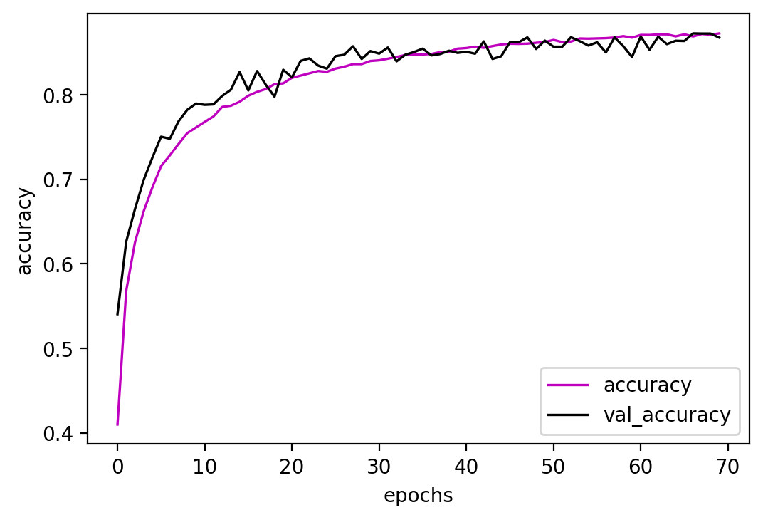
As explained before, the best non-overfitting model is the CNN-64, with 87% of accuracy on the training, validation, and test sets. Figure 3 shows the validation and training accuracy for each epoch.
The script cnn.py can be used to train either the CNN-64 or the LeNet-5 models on the GTZAN datasets.
python cnn.py train ../data/genres -v -m cnn64 to use the CNN-64 model, or python cnn.py train ../data/genres -v -m lenet. The training parameters and how to slice the data can be easily changed directly from the variables in the script.
The script can also be used to make use of the pre-trained models available in /models/ to predict the genre of one of the songs:
python cnn.py predict ../data/genres/ -f ../data/genres/rock/rock.00039.wav -m cnn64, -m being the flag showing which model to predict from.
The notebook: CNN.ipynb shows an example of how to train the model, read the data, etc.
Future Work – Lessons Learned
How did I get here?
This has been the work of several days of learning, of making mistakes, tweaking the parameters, and creating pretty cool solutions. While the solutions are easy once portrayed in front of anyone, I believe that it’s interesting to know how I arrived there, and what mistakes not to make in the future.
- Normalize the data: I can’t stress this enough. I was getting poor results the first day because I had forgotten this key step. Otherwise it’s very complicated for the network to learn when different attributes have totally different scales.
- Overfitting: Deep neural networks tend to overfit on small datasets like this one. How to solve this? through data augmentation, adding regularization. When the network overfits on the training dataset that means that it can’t generalize well to new dataset.
- Learning rate: I have tested 0.001, 0.0001, 0.0007, 0.0005. I would recommend using the default one, 0.001, unless you see oscillating loss values between epochs, in which case it can mean that the learning rate is not small enough.
A very good thread on this: link.
What is left? I would like to try and see if pre-trained networks on imagenet such as ResNet or VGG16 end up giving a good result on this problem. I have tried running ResNet50 pre-trained on ImageNet and it was getting ok results, though overfitting, and it seemed like an overkill for this kind of project. I believe I can get a higher validation accuracy on the LeNet architecture, but I leave that for future improvements.
References
[1] LeCun, Yann, et al. “Backpropagation applied to handwritten zip code recognition.” Neural computation 1.4 (1989): 541-551.
[2] Krizhevsky, Alex, Ilya Sutskever, and Geoffrey E. Hinton. “Imagenet classification with deep convolutional neural networks.” Advances in neural information processing systems 25 (2012): 1097-1105.
[3] Hochreiter, Sepp, and Jürgen Schmidhuber. “Long short-term memory.” Neural computation 9.8 (1997): 1735-1780.